Very fine 2D Modeling
Written by Chris Goodell | November 14, 2019
I’m a big fan of testing HEC-RAS to the limits. What can it do? What can’t it do? These are questions we should all ask at the beginning of a project. Can HEC-RAS actually prove to be a useful tool in answering hydraulic-related questions for our specific problem? Shortly after coming to work at Kleinschmidt I was posed with the question, “Can we use HEC-RAS to model a nature-like fishway? And more specifically, can we extract data from HEC-RAS to inform us of velocities and shear stresses between the many boulders and in the many pools that make up such a complicated feature?” The answer was YES! Check this out:
Here’s an example of making HEC-RAS work at a very small cell level, in order to get detailed results for design considerations.
And a zoomed in view:
The fishway is constructed using 11 concrete weirs and is approximately 300 feet wide by 400 feet long. The boulders are approximately 5 feet in diameter, with 2.25 feet projecting above the crest of the weirs. The gaps between the boulders range from 3 to 5 feet. In total, there are over 700 boulders in the fishway.
For the simulation shown, the drop from normal pond to the tailwater downstream of the last weir is approximately 6.4 feet or 0.58 foot per pool. The fishway is passing 890 cfs, 237 cfs of which is spilling over the top most weir from the headpond and the remainder is being supplied by 5 overflow gates. The 5 gates have varying levels of submergence on their tailwater sides, depending upon each one’s location, and they are each passing from 108 to 137 cfs. The velocity varies throughout the fishway, but is generally less than 6 feet/second. The nominal cell size in the mesh is 3 feet but decreases to 0.75 foot on the tops of the weirs to capture hydraulics between the boulder gaps. The largest cells have sizes of 96 feet and are located primarily in the headpond away from the fishway.
The model is run using the full momentum equation, with an eddy viscosity mixing coefficient of 0.44. The computational timestep is 0.1 second and the Courant Numbers max out at around 0.6, with the highest values being in the cells on the downstream sides of the gates where water is flowing into the fishway. The timestep is very small, but the model does not need to simulate a very long time since it is a quasi-steady model, meaning there are constant boundary conditions (a constant inflow hydrograph at the upstream end of the model and a stage hydrograph at the downstream end of the model). The model achieves steady state in less than 1 hour of simulated time. Model run-times averaged about 3 hours.


Comments
Smith Paul
on March 12, 2021This answers exactly what I have been battling with. Thanks, Chris
Add Your Comment