


February 20, 2025
Full Momentum Episode 37: All Things Gates
Gates play a crucial role in hydraulic modeling, impacting water flow, flood control, and dam operations.
One of the most frustrating aspects of unsteady HEC-RAS modeling can be the model stabilization process. You know, you’ve gone to great lengths collecting the best survey/topo data and solid hydrology. Then you’ve painstakingly spent hours…possibly days entered all of that data only to find that once you press the “Compute” button, the model crashes. The dreaded “Red Bar”!  Sometimes you can get your simulation to complete without crashing, but the listed numerical errors are so high that you can’t with good conscience submit that as your final simulation. Either way, approaching an unsteady HEC-RAS model (especially a dynamic one) as a beginner with little experience and understanding of how to stabilize it can cause significant delays in your project and worse, completely blow up your budget. I’ve uploaded two HEC-RAS projects to the following Google Drive Site: https://drive.google.com/folderview?id=0B_s8OLJOgOi0YU92SGZQZm9raWM&usp=sharing
RawleyResUnstable.prj is an unsteady flow dam breach HEC-RAS project recently sent to me for help. Although the model ran to completion without crashing, it had unacceptably high errors.
RawleyResStable.prj is the fully stabilized version of the model with no numerical errors.
The following lists out the courses of action taken to stabilize the model. Feel free to download the “Unstable” and “Stable” models and try these techniques on your own. The links following some of these items will take you to more information about that particular technique.
1. Cross Section Spacing. The initial spacing was way too coarse. A visual check alone of the geometry schematic and profile plot should encourage you to investigate a finer cross section spacing.
Geometry Schematic
Profile Plot Samuels equation suggests anywhere from 15 ft to 50 ft spacing (depending on what bed slope you use). I interpolated to 50 ft for the entire reach. http://hecrasmodel.blogspot.com/2008/12/samuels-equation-for-cross-section.html
Notice in the following profile plot of the downstream end of the reach how the water surface at the boundary cross section is below critical depth (the red dot). This creates an overestimation of the water depth at the next upstream cross section, which in turns creates some instability over the next several timesteps.
The proper way to handle this would be to find out what is downstream of your model and select a boundary condition that best represents those conditions. In absence of downstream conditions, the 0.001 slope for normal depth provides a reasonable solution. Either way, this underscores the importance of moving your downstream boundary far away from your area of interest in your study reach. That way the errors that do originate from your downstream boundary assumption will have diminished to negligible levels before impacting your area of interest.
I added more cross sections by interpolating the steep slope at the upstream end of the reservoir (10 ft spacing).
Notice the energy spike is not completely gone, but it is much better. Refining the HTAB parameters (http://hecrasmodel.blogspot.com/2009/02/crazy-energy-grade-line.html), turning on mixed flow and bumping up n values will collectively take care of the rest of this (see numbers 8, 9, and 10 below).
This is problematic in RAS. Using the graphical cross section editor, I redefined the bank stations to get rid of this problem.
I readjusted the cross section HTAB parameters to reflect the new bank station definitions (I used the “Copy Invert” button for all cross sections). While in there, I maximized the resolution of the HTAB parameters by changing number of points to 100 and minimizing the increment as much as possible while still having full coverage of each cross section. http://hecrasmodel.blogspot.com/2009/02/crazy-energy-grade-line.html http://hecrasmodel.blogspot.com/2011/03/more-on-htab-parameters.html
These are areas that are near critical depth. I turned on the “Mixed Flow” option in the Unsteady Flow Analysis window, which helps stabilize the near critical depths at the upstream end of the reservoir. http://hecrasmodel.blogspot.com/2011/04/mixed-flow-regime-options-lpi-method.html If you’ve been following along correcting your own copy of the model, you’ll notice that the model now finally runs to completion without crashing. There are still a few minor errors as shown in the Computation Messages.
It’s debatable whether you need to take care of these relatively small errors. Particularly for a dam breach model, where the presumed errors of the input data probably far outweigh these small numerical errors. Nevertheless, there’s a sense of pride in putting out a very robust model, completely free of numerical errors. So…let’s continue.
The section at the upstream end of the reservoir is very steep at about 13.5%. In fact, that’s greater than the suggested maximum slope of 10%, as stated in the HEC-RAS manuals. You can see as the pool starts to lower, the steep reach is exposed and because of the low n values, the water surface is calculated to be supercritical. Let’s assume that the geometry is correct, and the upstream end of the reservoir really is that steep. Jarrett’s Equation suggests very high n values should be used here (~0.2), based on the bed slope and hydraulic radius (after the breach when the reservoir has drained). The original model had 0.07 and 0.035 for the overbanks and main channel, respectively. I changed all the n values in this steep reach to 0.15, because I think 0.2 might be a little overkill. http://hecrasmodel.blogspot.com/2009/12/n-values-in-steep-streams.html
There…no errors! However, there is still a Warning about extrapolating above/beyond the rating curve at a bridge (R.S. 277).
There we have it. A clean solution. No errors, no warnings.
Comments
The comments are closed.