***Update: I received a few very important comments about this post that I want to share.
First, and this is very important: These methods are not meant to be used to do any kind of detailed bridge design or bridge scour analysis (contraction, abutment, or pier scour). The methods I present in this post are strictly as a means to include a bridge in a 2D area to gage its effect on the overall resulting flood inundation. Meeting FHWA standards for bridge modeling requires much more information than these options will provide you.
Second, Mark Forest posted a couple of very good comments that I would like to share. Please read his comments at the end of this post. There have been a lot of requests for examples of how to model bridges in 2D areas. First, let me state up front that in the current version (5.0.1) there is no direct way to put a bridge in a 2D area, like you would in a 1D reach. That means, that we currently don’t have a way to use low flow bridge modeling approaches like Energy, Momentum, Yarnell, and WSPRO. Likewise, you can’t use the high flow approaches (Energy, Pressure/Weir). Hopefully this will be added to a future version.
That being said, I’ll present three options for simulating bridges in 2D areas. To demonstrate these options, I used a dam breach model adapted from HEC’s Bald Eagle Creek data set. The animation is included at the end of this article.
Option 1. Simply modify the terrain to include the bridge embankments, abutments, and even piers. This requires a little work in GIS manually editing the terrain to include those features. If you have a RAS model and you don’t want to get into GIS at all, this is probably not the right method for you. However, if you are modeling an existing bridge, look closely at your terrain. You might see that the bridge components (minus the deck and piers) are already in there. When processing LiDAR data, it’s common to remove the bridge deck, but leave the roadway approaches and abutments. This may be sufficient enough, especially if the depth of water doesn’t get high enough to impact the bridge deck and there are no piers, or they are relatively small compared to the bridge opening. In this case, RAS will just use the regular 2D St. Venant equations to model flow through the bridge opening.
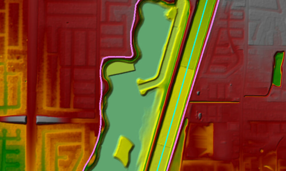
Here’s an example that shows a bridge that could be modeled using Option 1.
Notice the bridge deck appears to be inundated. Don’t be fooled by this. The deck is actually higher than the roadway approaches (which are dry), but since it’s not included in the terrain, RAS doesn’t know it’s there-it only sees the roadway approaches and the bridge abutments (see next figure). The deck is in fact not impacted in this case. Since the deck is not impacted, we can model this bridge using the existing terrain. In this case RAS will use the 2D St. Venant equations to compute stages and flows through the bridge opening. I’m not sure if there are piers under this bridge or not. If there were, you could either ignore them (if they’re relatively small) or try to work them into the terrain somehow. I suppose if you really wanted to get crazy you could make a very small 2D area connection for each pier, or even use very high n values in the cells that the piers occupy.
When setting up your geometry to model this as a bridge, there’s really not much to it. You are basically using the existing terrain and laying a mesh on top of it. However, it is important to establish cell faces along the top of roadway, since it will be acting as a barrier to flow. You can easily do this by drawing and enforcing breaklines as shown below with the red polylines.
Advantages:
Easy to set up for existing bridges that are included as part of the terrain.
Disadvantages:
Requires manually editing your terrain if you want to model a proposed bridge.
Can only simulate low flow through a bridge (can’t impact the bridge deck).
Can’t simulate piers.
Option 2. Use a SA/2D Area Connection with a culvert (or culverts). This is particularly useful for wider bridges with relatively small openings when the bridge deck is impacted during the flood. If the bridge has piers, you can use multiple culverts, the spacing between them is what simulates the piers. In this example (same HEC-RAS dataset), you can clearly see that this bridge, its abutments, and its roadway approaches are overtopped by the flood.
Here I’ve inserted a SA/2D Area Connection for the bridge.
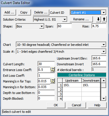
Although it is technically a bridge, we can simulate it with a culvert by using a box that has the same width and height as the bridge opening. Simply measure the width and height of the bridge opening and use that for the span and rise of the box culvert. I grabbed the dimensions of the bridge opening from the 1D version of the Bald Eagle dataset (converted from English Units). Try to get this as close as possible, although you’ll not get it exactly the same.
Although this is relatively easy to do, especially if you have the bridge dimensions on hand, it would be wise to calibrate this to the original model. Since bridges can’t be used directly in 2D areas, you’ll have to do your calibration in a 1D version of your model. Typically you’ll focus on the inlet coefficient, n values and the culvert width (span) as your calibration parameters. Try to replicate the stage hydrograph as closely as you can (this is usually difficult to do), but at least calibrate to the timing and water surface elevation of the maximum inundation.
Advantages:
Can simulate low flow and high flow conditions (i.e. bridge overtopping).
Disadvantages:
Uses culvert equations to model a bridge.
You may not be able to get the culvert shape to perfectly match the bridge opening.
Requires calibration.
Option 3. Use a SA/2D Area Connection with a gate (or gates). This is particularly useful for narrower bridges with relatively large openings when the bridge deck is impacted by the flood. If the bridge has piers, you can use multiple gates, the spacing between them used to simulate the piers. In this example (again…same dataset), it’s hard to tell if the bridge overtops, since there are some dry areas on either side of the deck. However, it is close. And if there is any thickness to the deck at all, it is likely that there will at least be pressure flow. We’ll verify this later.
Again, I’ve inserted a SA/2D Area Connection for the bridge.
From here, the technique is very similar to Option 2, only you’ll use gates instead of culverts. Again, get the dimensions of the bridge opening and use that to size the gates. In this example, there are two piers, so I’ll put in three gates (the space between the gates simulates the piers).
Here’s the bridge as it is input to the 1D version of the Bald Eagle dataset:
…and in the 2D model using gates:
To simulate the two piers, I had to create three different gate groups, since the resulting openings are all slightly different.
One unique consideration for Option 3 is that you have to add time series boundary conditions for operation of the gates. It’s easy to do, you just have to create a new unsteady flow file and add in the boundary conditions. Just set the gates to be fully open for the entire simulation. And don’t forget to set the time series for all three gates. You’ll get a somewhat unhelpful message if you do forget.
As with culverts, it’s important to calibrate your gate version of the bridge to the bridge in the 1D version of the model. For gates, you’ll want to focus on the weir coefficient and the sluice discharge coefficient as well as the width of the gates for your calibration parameters.
Advantages:
Can simulate low flow and high flow conditions (i.e. bridge overtopping).
Disadvantages:
Uses gate equations to model a bridge.
You may not be able to get the gate shape to perfectly match the bridge opening.
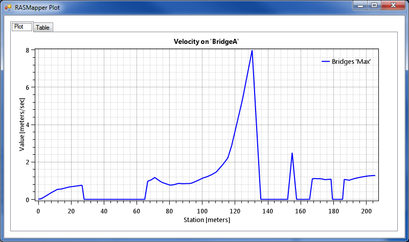
When checking output, you will get stage and flow hydrographs for the two methods that use SA/2D Area connections. However, you’ll find they are generally not too useful-they’re geared more towards presenting 1D simulation results. In 2D areas, I prefer to use the Profile Lines. Below, I plotted both the maximum water surface elevation on the terrain profile as well as the velocity profile. If you revisit the plot shown above of the SA/2D Area Connection that represents this bridge, you’ll see that the bridge deck upper chord is at an elevation of approximately 174.3 meters. And the lower chord of the deck is approximately 173.2 meters. Therefore, the bridge doesn’t overtop during the simulation, but it does go into pressure flow.
Also, you can clearly see that the right bank will get some potentially damaging velocities! (This is after all, a dam breach simulation).
It’s interesting-this velocity hotspot is not what you might think. I initially assumed that this was velocity in the direction of the creek, moving “downstream”-the velocity we typically consider when determining abutment scour. However, when plotting the particle tracing and velocity vectors on top of the water surface elevation layer, you can see that this is actually high velocity from water spilling over the bank (again, this is a dam breach model, which is why you have water spilling from the overbank into the channel). The drop in water surface elevation over the bank is about 3 meters!
Here is a zoomed-out view of the dam breach flood event. Look closely during the animation-the cursor points out the three bridges that were modified for this article.
Do any of you have any other ways to model bridges in 2D areas? If so, please share!
Mark Forest, Practice Leader – Floodplain Management and Modeling at HDR Engineering has the following to add: “That is a good summary. I would note that if you include the piers in the terrain, it is important to build breaklines through the piers and use a small enough grid spacing around the piers if you want them to be properly simulated as obstructions to the flow path. Otherwise they just displace volume. Also, the impact of the piers really requires the full momentum solution as well. The run-up on the face of the pier will be seen with the full momentum solution when properly gridded around the pier. Also, when you are attempting to simulate flow around the abutments (that you have carefully incorporated into the terrain), it will require a finer mesh around the abutments to capture the more detailed velocity distribution in that part of the model domain.
Non-pressure flow bridges can be effectively modeled this way, if the terrain has been properly captured.
I would also note that, the region under a bridge deck is not going to be properly captured with LiDAR data since the bridge deck obscures the returns. This usually leaves a “hump-like” feature in the LiDAR data set under the deck. This has to be manually cleaned up in order to model this with 2D. With a 1D model this is not typically a problem since you are extracting the sections for the bridge faces outside of the zone of bad data. But, with the 2D solution, that hump under the deck will be seen as an obstruction to flow through the opening.”

 There have been a lot of requests for examples of how to model bridges in 2D areas. First, let me state up front that in the current version (5.0.1) there is no direct way to put a bridge in a 2D area, like you would in a 1D reach. That means, that we currently don’t have a way to use low flow bridge modeling approaches like Energy, Momentum, Yarnell, and WSPRO. Likewise, you can’t use the high flow approaches (Energy, Pressure/Weir). Hopefully this will be added to a future version.


Comments
The comments are closed.