
February 20, 2025
Full Momentum Episode 37: All Things Gates
Gates play a crucial role in hydraulic modeling, impacting water flow, flood control, and dam operations.
Fortunately, hardware aside, there are some advantages that are not well known built into HEC-RAS that we can use to significantly reduce run times without needing to compromise on model stability. We can also get the same consistent and reliable outputs we all count on. The future of the discipline is moving closer and closer to the cloud as technology and rapid software development for information-technology operations (DevOps) cut development lifecycles for new engineering tools ever shorter. Many engineering firms are already finding ways to bring engineering workloads to the cloud through virtualization. To save money and leverage important resources our creative solutions need to consider computational efficiency and performance as well as tie those metrics to estimates of cost and public good.
This article demonstrates the use of adaptive time steps in HEC-RAS and presents an easy-to-use method for determining time step divisors for highly dynamic flood events. As an example, I recently finished a single mesh 2D HEC-RAS model for floodplain mapping. It contained 868,000 cells and simulates a 24-hour rain-on-grid event. The method I will explain in this article reduced the run time from 49 hours to 4 hours, a reduction of 91%! The table and plot below summarize the results.
| Statistics | Original Run Stats | Modified Run Stats | Delta | Delta by Percent |
| Computation Time Total | 49:31:59 (h:m:s) | 04:17:35 (h:m:s) | – 45 hours | – 91% |
| Vol Accounting Error | 28.43 (acre-ft) | 44.96 (acre-ft) | + 16.5 (acre-ft) | +58% |
| Vol Accounting Error Percentage | 0.054% | 0.080% | + 0.026% | +48% |
| Example Azure Cloud Cost | $ 17.89* | $ 1.54* | $ 16.35 | – 91% |
*Note: Azure instance was assumed to be containerized (usually docker) set with 6 GB of RAM and 4 vCPUs (would not increase further in online calculator). Costs may not represent reality, but ratios may be informative. Also, containerized storage was also not considered.
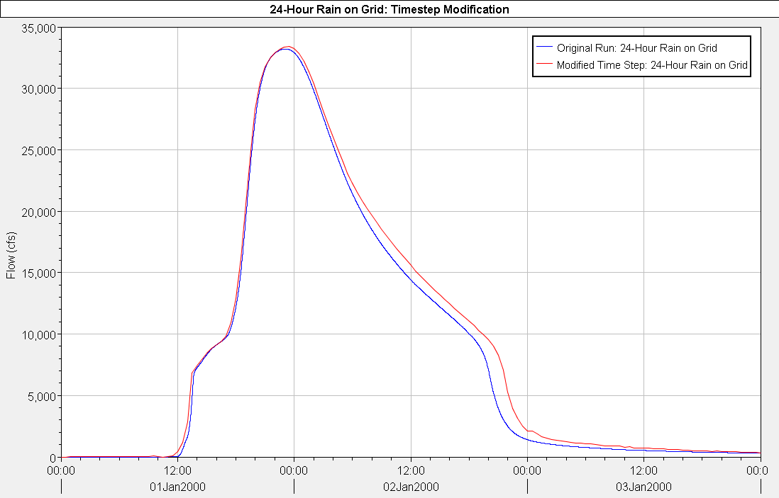
In the figure above, notice how closely the two hydrographs match versus the amount of computation time needed to generate the output hydrograph. Level of definition, of course, should be considered with your project type, public safety and your client.
In the case above I did not have any observed data to calibrate to, so I cannot make any determination of which hydrograph is more correct. The difference is negligible anyway.
If you were at any point concerned with model stability, then you are familiar with the Courant condition. You might also see it as the Courant–Friedrichs–Lewy Condition (CFL) if you google it online. I won’t go into it here, since there are already many resources online, but I will save you some time by saying that RAS is not like most other Hydraulic models, so what you find online may not be directly applicable. The key element is that RAS uses an implicit solving scheme rather than an explicit scheme. Generally, this means that a higher courant number can be used rather safely and still have stable outputs. In fact, this is by design. The excerpt below is from the RAS Hydraulic Reference Manual.
Implicit Finite Difference Scheme
“The most successful and accepted procedure for solving the one-dimensional unsteady flow equations is the four-point implicit scheme… For a reach of river, a system of simultaneous equations results. The simultaneous solution is an important aspect of this scheme because it allows information from the entire reach to influence the solution at any one point. Consequently, the time step can be significantly larger than with the explicit numerical schemes.”
From: CPD-69 Ch 2: 2-29-30
While the excerpt above is from the 1D Unsteady section, RAS’s 2D equations and methods are built atop of them. Let’s break this excerpt down because it says quite a bit.
When choosing a timestep the key, traditionally, is to achieve a numerically stable model. But it is also equally important to make sure that the timestep is small enough that the chances of missing the peak of the wave at a sampling point (Cell face or XS) is small. RAS, at every computation interval, looks at the whole grid (sparse matrix of linear equations) and solves for what it expects to see (a dynamic wave). You have a lot of opportunities to characterize the flood wave with your chosen computation interval. But, does the value of that opportunity change throughout the simulation? If so, how can we take advantage of it?
To illustrate that last point further, consider a different but very related example; converting analog music to digital. Look at the graphic below. A computer samples the wave at a regular interval. These would be the vertical periodic red arrows. You might intuitively know that many arrows corresponding to a sampling point, or time the wave was measured, would result in more dots to interpolate between. Less arrows results in less points and the wave loses definition.
Can we have too many arrows? More does mean better quality, but that higher quality can become meaningless if you are sampling the wave for qualities greater than what any human ear can discern. In the figure below I highlighted a couple places where we might be able to take advantage of a dynamic sampling method. Dynamic sampling would basically optimize arrow placement to a wave shape objective function. You might equate this to running a RAS model at a constant 30 second interval vs advanced time step control which would try to use the CFL condition at each time-step to adjust it for you automatically. The dynamic sampling tries to reduce the overall number of samples taken by sampling more where you need it and less where you don’t.
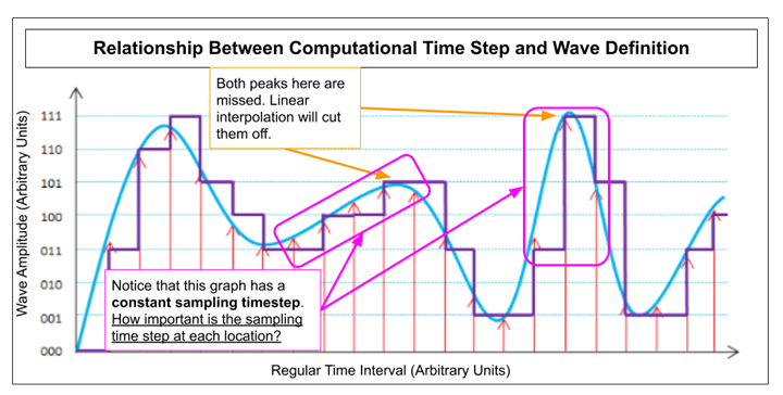
Notice that sampling does not need to be at a regular interval to accurately reproduce the wave later. In RAS, we just need to know when in your simulation you will need more definition and when it is less important. Just using a small Courant value may ensure that your simulation does not accumulate errors but will ultimately serve no purpose but to test your patience.
Just to check in, you are probably now more fully convinced of something you already know. Don’t use a fixed time step, use the automatic one based on the Courant condition. Unfortunately, these settings are not usually set correctly and frequent spikes in the calculated Courant condition (C) value on the grid can slow the whole model down for periods that are less important in time. I think the most effective method for setting time step is based on time series of devisors.
As you will see, your intuition of the models needs can be much sharper than a simple function that samples the whole grid indiscriminately at each time step. Until RAS increases the sophistication of the Courant based time step program, you can easily do a better job being the dynamic controller of your model for simple cases.
To optimize our models, we will need two things. 1) A way to easily calculate and apply a C value and, 2) a method for predicting when we will need densely or sparsely sampled points. 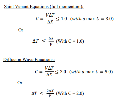 To do this, we will break up the simulation run into Hydraulically Important Periods or HIPs. This will help us predict what is happening between boundary conditions. Fortunately, guidance given in the RAS manuals helps solve the first problem. See the figure to the right (From: HEC-RAS 2D Modeling User’s Manual: page 4-5).
To use these equations, you need to make assumptions about V or velocity of the flood wave (wave celerity also refers to the speed of wave propagation). This will need fine tuning in the future but a great place to start for flatter watersheds is 5 ft/s. Steep watersheds or breach events will need something like 10 ft/s. Please note, I haven’t tested higher velocities as much as lower ones. These are rough estimates that have worked well with flood mapping exercises.
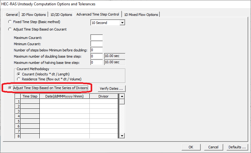
For applying the desired C value at various HIPs, we will use the advanced time stepping window. For the unsteady solver look for “Adjust Time Step on Time Series of Divisors” section. Don’t worry I will show you in more detail below. However, if you have any doubts about where we are in the process then see the hint that was left in the RAS documentation below.
The Time Step Divisor method for controlling the time step requires much more knowledge by the user about the events being modeled, the system being routed through, as well as knowledge of velocities, cross section spacing, and 2D cell sizes. However, if done correctly, this method can be a very powerful tool for decreasing model run times and improving accuracy. From: HEC-RAS Supplemental to HEC-RAS 5.0 User’s Manual: Page 2-8.
For some of you your intuition might have noticed that velocity is not necessarily the same as celerity. You are correct. To remove any confusion going forward I want to highlight a couple important definitions to help keep everything in order.
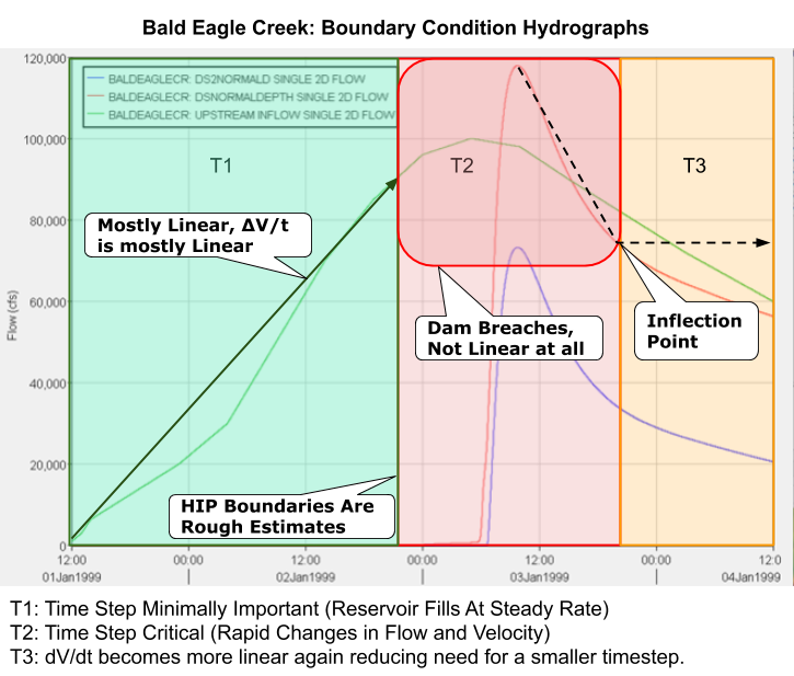
There are a number of ways to improve this method, but it will only complicate the basic concepts which are already very powerful and produce impressive results. In the example below I am using an output hydrograph (since the model was given to me) but an input hydrograph or hyetograph, for rain on grid, could help you establish a reference and the basic parameters of the estimator model we are building. The goal is to separate the model simulation into Hydraulically Important Periods (HIPs). We are taking advantage of the expected temporal variability to discretize the simulation into time zones and dynamically sample our flood wave ourselves. What we are concerned with here are the periods in the simulation where the velocity of the flood wave is or is not changing rapidly as it moves downstream.
The example below comes from the Bald Eagle Creek Dam Break sample dataset included with RAS. Since it is a dam break simulation, we already know there will be a period where the dam fills, a breach event and propagation downstream followed by a gradual recession of floodwaters. In the example below I want to look for any information that I can use to determine these period windows during the simulation. These periods and their boundaries will be our three HIPs. Modeling other hydraulic conditions may result in a different number of HIPs. What you choose is dependent on model conditions but you should aim to separate your simulation into time zones where your model will need more sampling to accurately produce the predicted flood wave as it moves downstream.
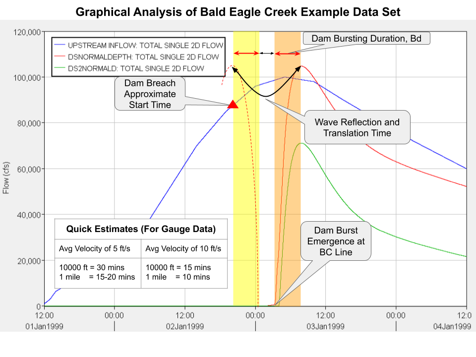
I personally like to start with the most intense event and work out. In this data set a dam fills and then breaches at a certain water surface elevation. Since time is not given, we are left to choose some form of rough estimation. There are a variety of ways to make estimates. The one below is perhaps a more elaborate example than necessary, but I wanted to highlight something interesting for this post. Below we are looking at a blue input hydrograph and two downstream output hydrographs from the 2D grid. I want to concentrate my computing power on the most dynamic parts of the event. Ideally, this will be from when the breach starts to about when floodwaters begin a gradual decent at the model boundary.
Looking at the downstream hydrographs we know that they are a reflection (along the y-axis) of the dynamic wave that the breach generated upstream. Fortunately, they are well defined due to a significant travel time. Choosing the downstream peak as a reference point, we can roughly rewind time at an estimated 10ft/s for 100,500ft (approximate distance between outlet and breach point) for a back calculation of roughly 3 hours. This can be estimated graphically as shown below. You can choose to carry out the calculations, but it is not necessary. This middle zone where the dam breaches and the primary flood wave moves downstream is where I will concentrate RAS’s computing power with a smaller time step.
Once the critical part of the simulation has been identified then we are looking for when to establish the boundaries for HIPs one and three. Boundaries of the primary event are clear and looking for inflection points can help for finding a good drawdown boundary. Just keep in mind that highly dynamic periods, where velocity is changing rapidly, will need more time-steps. Input hydrographs, precipitation, gauges, etc. give great clues but are all translated in time.
This example is based on the Bald Eagle Cree Example Dam Break Study Dataset which is included with the installation of HEC-RAS. This example is meant only to illustrate methods proposed above.
Our goal will be to use the HIP model optimize time step to reduce overall run time without sacrificing model stability. Model stability will be characterized by the following criteria:
Below is a summary of the base run as provided by USACE on specific hardware
| Default USACE Settings | Base Run Statistics |
| Grid Cell Size
Cell Count Simulation Time Window |
250×250 ft
~19600 4 Days |
| Computation Task Time(hh:mm:ss) | 4:10 |
| Error
Percent Error |
6.826 acre-ft
0.001791% |
| Hardware Summary | 3.8 Ghz
10 Cores/20 HT Cores M.2 Solid State Drive |
Our goal is to gain some insight as to what is happening, in time, between boundary conditions in order to better predict what our model needs computationally and when. Fortunately, we have the results from this run already. If that were not the case I would just estimate graphically as shown earlier or do a quicker rough run with a larger time step and larger grid cell size.
The dam break example is set to breach at a specific water surface elevation. Without running any plan initially, we would only have the green inflow hydrograph below to make our estimate. Having already run the default model to ensure it was working properly and looking at some of the outputs, I know that this is not enough.
Strategy: For complicated scenarios it may be beneficial to run the model with a larger grid size and timestep to get a better idea of what is happening along your study area. The default setting for this plan resulted in a run time of 4:10s. I think the value gained in a rough run is well worth it. Just make sure to stay within the recommended limits of the given equations so you don’t introduce other unknown factors. From personal experience I can say that if C is too low or much too high errors can quickly accumulate on the grid causing it to iterate on cells with too much error. This can easily get out of control and cause your simulation run time to take much longer. It helps sometimes to lower RASs iteration count to something like 5-10 to nudge RAS to go unstable and quit. If your model is frequently hitting 10 iterations on cells in your model it is best to stop and double check what is going on. You can use RASs restart options if you really need to save time.
With some iteration, I established the following HIP zones for my study area. Unfortunately, I didn’t think about the graphical method I showed earlier until after. It would have saved me a bit of time!
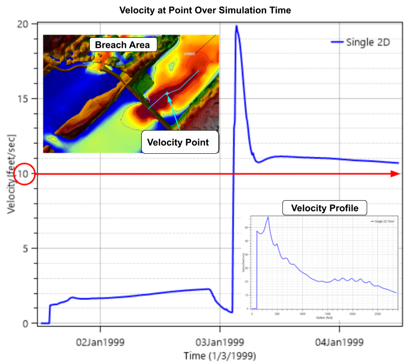
The equation we are using is reproduced below (From: HEC-RAS 2D Modeling User’s Manual: page 4-5). With grid size already fixed at 250dxdy we need to estimate velocity. Along a normal reach I would simply use 5 ft/s as a starting point. 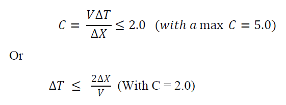 However, the dam breach is likely to exceed that significantly. Drawing a profile line just downstream of the breach with max velocity layer turned on I can sample that surface with the line in RAS Mapper. The location of that line and the sampled velocity profile are below. You can see that I roughly choose 10 ft/s.
Choosing a good C value is much like you might already be used to. However, remember that RAS uses an implicit solver. I generally choose C values between 3-5 and only go lower when it is really needed. In a breach case we need to keep C a bit lower to maintain stability. A summary of the calculations is below.
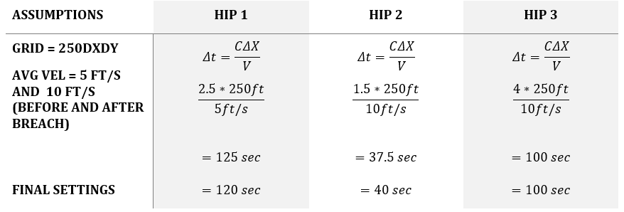
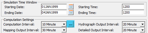
1. Set Computation Interval to 10 min (Some multiplier > than HIP 1)
Note about choice of computation Interval: The computation interval you choose can limit the number of time divisors you can use in a HIP. To save someone a headache, just remember that larger computation intervals will allow for more fine tuning in your desired time step.
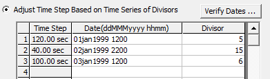
2. Adjust Time Divisors (See below for an example)
Access the table of time step divisors by clicking on the ellipses (…) next to the time step dropdown box in the figure above. Note about divisors: The divisors can be a little confusing at first. The first line must be equal to the start time of your model. RAS continues with this first-time step until it meets another time step definition and so on. The last line will simply be used until the model simulation ends. The divisor is then the number to divide the computation interval by to achieve the desired adjusted time step. For example, for HIP 1, 10 minutes (600 seconds) divided by 4 equals 150 seconds.
3. Compare Results
| “Out of the Box” USACE Settings* | Base Run Statistics | Modified Time Step | Delta |
| Computation Task Time(hh:mm:ss) | 4:10 | 2:11 | 49% |
| Error
Percent Error |
6.826 acre-ft
0.001791 % |
3.098 acre-ft
0.000812 % |
54.6% |
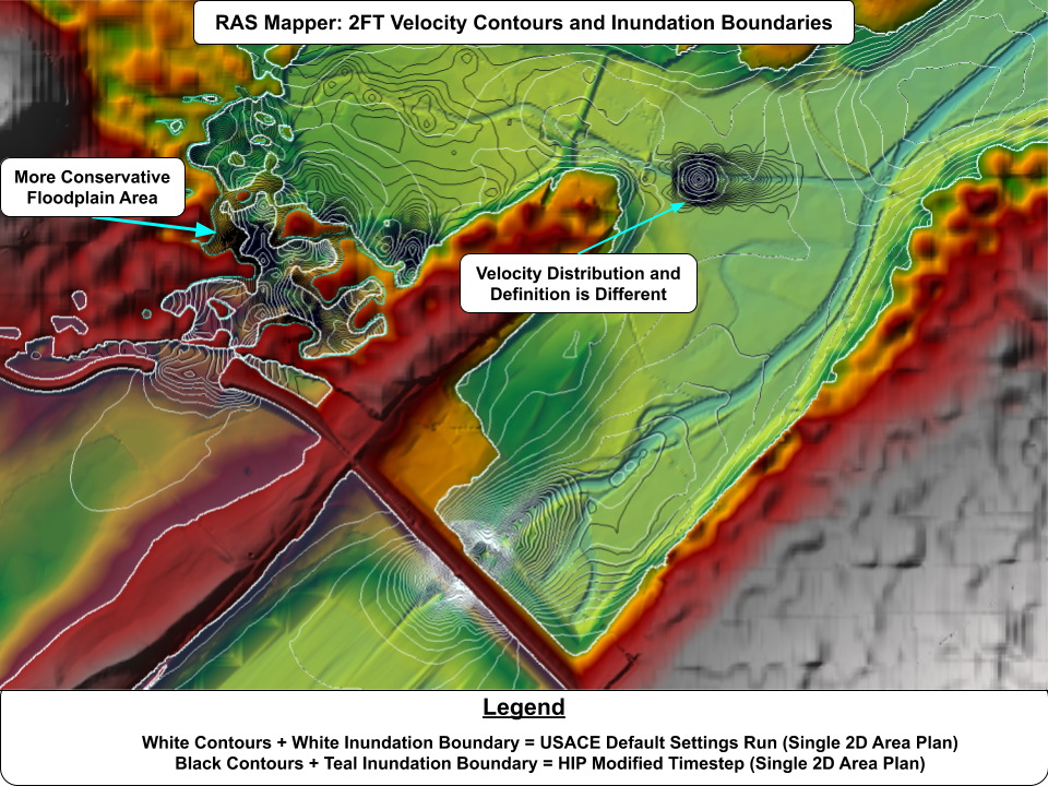
The results show that using the HIP model for adaptive time stepping reduced both the computation time and volume accounting errors by around 50%. Below I show both results maps superimposed. We can see that the adaptive time stepping produced a slightly more conservative floodplain boundary near the spillway. We also notice some significant changes to the velocity contours downstream of the Dam as well. It is interesting to see what could be argued as more definition in the modified run than the original even though the smallest timestep in the modified run (40 seconds for HIP2) was still greater than the 30 seconds for the default run. I am interested to see what reasons the community can come up for why this is.
For the two hydrographs below, downstream boundary and breach, I just want to highlight how similar the solutions are to both models with and without adaptive time stepping. RAS was designed with some powerful tools allowing us to reduce runtimes while keeping results consistent.
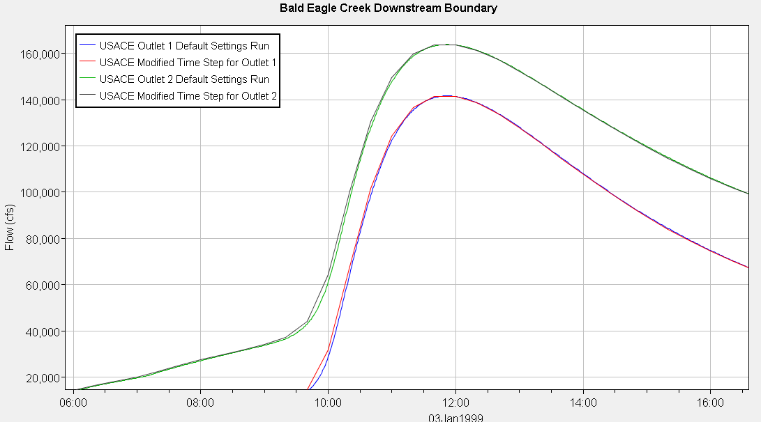
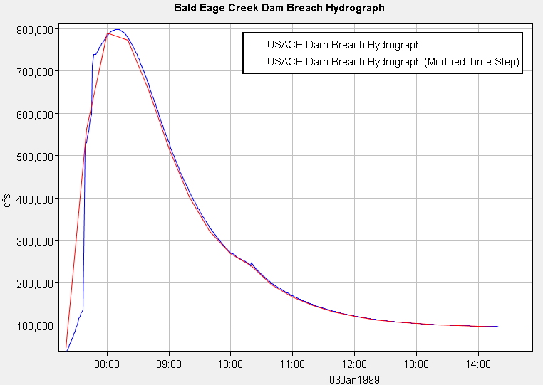
The downstream boundary hydrographs are shown here for both simulations. If you are interested in peak discharge you can see here that the adaptive time stepping does not significantly impact model precision. Both hydrographs are within 50 cfs of the original run. The real danger of larger time steps is move evident in the breach hydrograph below. You can see that the peak of the original run lands between timesteps. Still, the difference in peaks is less than 3,000 cfs and amounts to a 0.004% reduction over the original run.
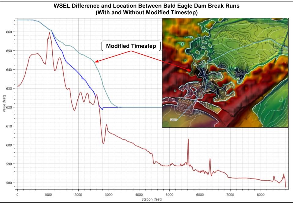
The final figure below shows a drawn polyline in RAS Mapper through the spillway to show differences in WSEL between the two runs. Some of the differences there might be alarming but keep in mind that this dataset was only intended to show what RAS CAN do rather than an example of how it should be done. The LiDAR there is particularly coarse among other things. Casual visual inspection of the rest of the model showed no discernable differences between inundation boundaries or velocity contours.
This method focused on classifying shallow wave propagation into Hydraulically Important Periods (HIPs) or changes in time. With modification this method can be adapted for other use cases. However, there is still changes in space to explore for further optimization. These will more heavily focus on RAS’s special grid features which are also rather unique to RAS.
Lastly, while it might be easy to intuitively modify the method for alternative use cases, please don’t forget the simplifying assumptions we are making. Understanding those will help anyone who wants to build on this.
Key Assumptions:
Key Concepts
Copyright © 2020 The RAS Solution. All rights reserved.
Comments
Cameron Jenkins
on October 2, 2020A few comments/questions on this.
1. I am glad this is being brought up as it can help speed things up if you understand your model.
2. Thanks for the write-up, it was an interesting read and I can tell you have spent some time looking into this.
2. HEC-RAS is a Semi-Implicit model not Implicit.
3. Orthogonal grid cells solve a lot faster than Non Orthogonal.
4. Optimizing your mesh so there are not a lot of iterations can also speed up your model significantly.
5. I have found that once you add in hydraulic structures such as culverts in the mesh, the model is more sensitive to the timestep.
6. Have you done tests with the different solvers (full momentum/diffusion wave) and this method?
7. Have you done tests with different cell sizes and this method?
8. In your tests, did you have any cells that had high volume iteration errors? Maybe around the areas where you showed the results were different?
9. Have you ever tried this with grid cells that are around 20 ft in size or a model with lots of hydraulic structures?
Chris Goodell
on October 2, 2020Thanks Cameron for you comments on this post by Jaison. I would say semi-implicit versus implicit is a bit more nuanced. RAS can be either. So in a sense you are both correct. RAS can use a semi-implicit solution IF you chose a theta weighting factor other than 1. Leaving your theta = 1 essentially makes it an implicit solution scheme. If you look through the manuals RAS sometimes calls itself implicit, sometimes semi-implicit, depending on what section you are reading. Of course we could have a discussion on the merits of changing theta, but in practice, most people leave it at 1. But good you brought that up, because I don’t think many RAS user’s understand this option, or the consequences of it.
Luis Partida
on October 5, 2020Hi Cameron, Could you elaborate a little more on your comment #4. More uniform cell shapes correlates to more consistent spacing therefore minimizing potential Courant numbers?
I too have currently been implementing adaptive time steps in a current 96 sq mi 1D 2D model and it has greatly improved performance.
Luis Partida
on October 5, 2020**Minimizing potential Courant number variances**
Isaac Thomas
on October 27, 2020My work computer has 4-cores. I have noticed that I consistently have about a 5% model run time reduction, when selecting “4 cores” instead of the default “All Available” under
Unsteady Flow Analysis >> Options >> Calculation Options and Tolerances >> 2D Flow Options
My models I have tested this on range between 100k to 200k cells, at 20′ x 20′.
I would be interested if other people following this blog notice a similar trend when specifically selecting the number of cores on their respective computers vs. the default “All Available.”
Chris Goodell
on October 28, 2020Thanks for sharing that Isaac.
Sauhard
on November 12, 2020Hey Everyone, Can anyone explain to me the point “larger computation intervals will allow for more fine tuning in your desired time step.” in the article. I could not understand what it meant and how.
Chris Goodell
on November 17, 2020By starting with a larger global computation interval, you’ll have more room to subdivide it using the time series of divisors.
Diana
on November 16, 2020Hi Chris, Im a final year civil engineering student and I’m using HEC-RAS to create flood maps for my final year project. I have extensively done my reading and googled my way around but there is one thing that seems unclear to me. In order to create flood maps, is it possible to do so with only Hec-RAS since the creation of RAS Mapper in the 5.0 update? Or would I still need a GIS software like ArcGIS or QGIS?
Chris Goodell
on November 17, 2020Hi Diana. While RAS Mapper will allow you to create a flood map on its own, RAS Mapper is still somewhat limited in its utility when compared with ArcGIS or QGIS. You don’t necessarily need a GIS software, but you may find it useful to put together really nice maps. Good luck in your final year! Keep an eye on our job postings at Kleinschmidt!
Hassan R
on November 20, 2020Hi every body!
Thank you Jaison for the post and Chris for answering our questions.
I still have some difficulties for selecting my appropriate time step. Generally, when we solve problems numerically, the mesh independency should be conducted to lend credibility to the solution i.e. refine the mesh until the results don’t change significantly. I feel the same should be the case for time steps. But it looks like I am wrong! Time step is apparently more fragile. Jaison mentioned that how it is tied to the stability of our solution. Still, intuitively, I expect once I reduce the time step get better results, but I don’t. For instance, the BC upstream hydrograph has a 6-min time step. I solve for 6-min computation time steps and for 30-min. The latter produces the correct results. For 6-min, the flood does not even reach the downstream. What am I doing wrong here?
Chris Goodell
on November 20, 2020Make sure you are following the Courant number guidance provided in the manual.
Hassan R
on November 23, 2020Thank you, Chris, for the suggestion. I will revisit the manual.
Matteo Marcelli
on March 16, 2021Good afternoon Chris,
I wonder if the primary event refers to the red downstream hydrograph and if so the secondary event would be represented by the green smaller hydrograph? Also, to which downstream sections do the two downstream hydrographs refer to?
Many thanks
Paqui
on July 26, 2021Hello Chris, I have a question. The main difference between using FIXED TIME ESTEP (BASIC METHOD) or ADJUSR TIME STEPBASED ON COURANT is simply the computation time since it can be reduced a lot. What I mean is that if until version 5.0.3 only the first option existed, the results provided by both methods are correct if the model is stable, it is simply that the first model needs to perform all the iterations, and is therefore much slower.
Many thanks.
Chris Goodell
on July 30, 2021Yes…sort of. It’s more that the first option would use a smaller time step for the entire simulation, so it would take longer to run. But yes, iterations do slow down your computations too.
Add Your Comment